이전 포스팅으로 XOR 문제를 해결할 수 없는 SLP와 이를 극복한 MLP에 대해 간략하게 설명했다.

이번 포스팅 부터는 딥러닝을 구현한 파이썬 코드와 개념, 그리고 베이스라인에 대해 설명하면서 진행할 예정이다.

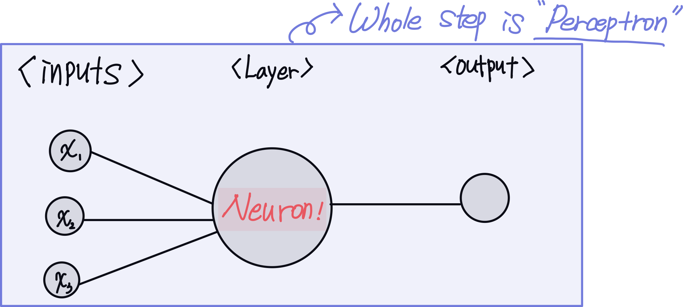
| 퍼셉트론을 이용한 딥러닝의 학습 과정

딥러닝 학습 과정은 먼저 아주 크게 두 갈래로 나눌 수 있다.

1) feed forward (순전파)

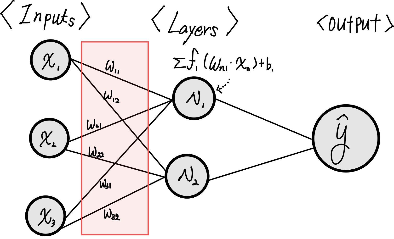
- 말 그대로 전진하는 것이다, 계산을 input → neuron → output 방향으로 진행되고 이 계산의 목적은 임의의 예측값인 y_hat을 도출하는 것이다.

- 모델이 학습되기 전에는 이 y_hat이 제멋대로인 값을 출력할 수 있다. (정답 레이블 또는 기대값이 100인데 15억을 출력한다거나)

2) Backpropagation (역전파)

- 역전파는 설명의 편의성을 위해서, 순전파의 반대방향으로 연산을 진행하는 것이라고 한다.  (맞는 말이긴 하지만 곱하기를 나누기로 하는게 반대다! 라고 생각하는 나 같은 사람한테는 맞지 않는 설명이라고 생각하며 아래만 보는게 더 와닿는 느낌이다.)

- 역전파는 순전파를 통해서 결정된 y_hat에 대해서 ①정답 레이블로부터 오차 크기를 계산해서 ② 순전파 계산에 활용되는 weight와 같은 파라미터들을 조정해 나가는 과정이다.

- 파라미터를 조정하는 방향은 파라미터가 total Loss에 미치는 영향에 대해 알아야 하므로, 편미분형식으로 진행이 되는데 상세히 설명되어 있는 wikidocs 문서를 참고하면 좋을 것 같다.

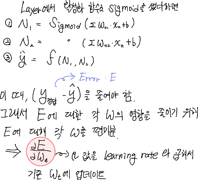
* learning_rate : 역전파 한 스텝 당, 얼마나 weight를 조절할 지에 대한 비율

| MLP 구현을 통한 딥러닝 학습 방법에 대한 이해

- 준비물 : 파이썬 3.6 버전 이상, numpy, pandas, matplotlib, seaborn, torch, scikit-learn

오늘은 가볍게 MLP를 통해 "tips" 라는 데이터 셋을 학습하도록 구성해본다.

tips 데이터셋은 seaborn라이브러리에서 제공해주는 어떤 식당에서의 결제/팁/결제자 정보를 담은 데이터셋이다.

1. 데이터셋 불러오기 및 확인

import pandas as pd
import numpy as np
import seaborn as sns

data = sns.load_dataset('tips')

data.info()
'''
<class 'pandas.core.frame.DataFrame'>
RangeIndex: 244 entries, 0 to 243
Data columns (total 7 columns):
 #   Column      Non-Null Count  Dtype   
---  ------      --------------  -----   
 0   total_bill  244 non-null    float64 
 1   tip         244 non-null    float64 
 2   sex         244 non-null    category
 3   smoker      244 non-null    category
 4   day         244 non-null    category
 5   time        244 non-null    category
 6   size        244 non-null    int64   
dtypes: category(4), float64(2), int64(1)
memory usage: 7.4 KB
'''

data.head()
'''
total_bill	tip	sex	smoker	day	time	size
0	16.99	1.01	Female	No	Sun	Dinner	2
1	10.34	1.66	Male	No	Sun	Dinner	3
2	21.01	3.50	Male	No	Sun	Dinner	3
3	23.68	3.31	Male	No	Sun	Dinner	2
4	24.59	3.61	Female	No	Sun	Dinner	4
'''

데이터셋을 불러오는 법과 구성은 위와 같고,

데이터셋을 통해 tip을 제외한 6개의 컬럼을 이용해서 tip을 얼마나 주었을 지 예측하는 MLP모델을 작성해보려한다.

2. 데이터 전처리

import torch
import torch.nn as nn
import torch.optim as optim
from torch.utils.data import DataLoader, TensorDataset

from sklearn.model_selection import train_test_split
from sklearn.preprocessing import LabelEncoder

device = torch.device("mps" if torch.cuda.is_available() else "cpu")

def categorical_encoding(col):
    encoder = LabelEncoder()
    data[col] = encoder.fit_transform(data[col].to_numpy())


for i in data.columns:
    if data[i].dtype == 'category':
        categorical_encoding(i)


x = data.iloc[:, [0,2,3,4,5,6]].values
y = data.iloc[:, [1]].values

x = torch.tensor(x, dtype=torch.float32).to(device)
y = torch.tensor(y, dtype=torch.float32).to(device)
print(x.shape, y.shape)

x_train, x_val, y_train, y_val = train_test_split(x, y, test_size=0.3, random_state=42)
print(x_train.shape, x_val.shape)

train = TensorDataset(x_train, y_train)
validation = TensorDataset(x_val, y_val)
print(train)

train_loader = DataLoader(train, batch_size=16, shuffle=True)
val_loader = DataLoader(validation, batch_size=16)
print(train_loader, val_loader)

* 맥북 M1 에어 모델에서 작성되어, mps로 매핑하였으나 cpu를 사용하려면 device구문을 제거하면 된다.

1) total_bill과 tip을 제외한 나머지 value들은(성별, 흡연 여부, 요일, 방 크기 등) 모두 categorical 데이터이므로, 레이블링 작업을 통해 모델이 학습 가능한 형태로 수정한다.

2) 그 다음 독립변수(x)와 예측할 종속변수(y)로 데이터셋을 구분해준 뒤, 사이킷런을 통해 학습에 사용될 trainset과 모델 검증에 사용될 validation set으로 데이터를 분할해준다. (비율은 통상적으로 7:3)

3) 모델 학습에 용이하도록 데이터의 형태를 변경해준다. 
- 텐서 데이터셋은 train set인 x_train, y_train 두 쌍을 하나의 데이터 셋으로 저장하고 인덱싱이 가능한 형태로 변경한다

- 데이터로더는 batch size를 조정해 추후 학습을 진행할 때 배치 단위로 전달할 수 있으며, augmentation, shuffle 등 다양한 기능을 지원하기에 수동으로 해야 하는 작업들을 보다 편하게 사용할 수 있도록 변경한다.

dataset = next(iter(train))
x_sample, y_sample = dataset
print("x sample: ", x_sample)
print("x sample shape: ", x_sample.shape)
print("y sample: ", y_sample)
print("y sample shape: ", y_sample.shape)

print('\n----- dataloader ----- \n')
# 첫 번째 배치 가져오기
first_batch = next(iter(train_loader))
X_batch, y_batch = first_batch
x_last, y_last = list(train_loader)[-1]

print("X_batch shape:", X_batch.shape)  # 입력 데이터(batch) 크기
print("y_batch shape:", y_batch.shape)  # 레이블(batch) 크기
print("X_batch example:", X_batch[:5])  # X의 일부 예제
print("y_batch example:", y_batch[:5])  # y의 일부 예제

print("last batch shape: ", x_last.shape, y_last.shape)


'''
x sample:  tensor([15.5300,  1.0000,  1.0000,  1.0000,  0.0000,  2.0000])
x sample shape:  torch.Size([6])
y sample:  tensor([3.])
y sample shape:  torch.Size([1])

----- dataloader ----- 

X_batch shape: torch.Size([16, 6])
y_batch shape: torch.Size([16, 1])
X_batch example: tensor([[ 9.7800,  1.0000,  0.0000,  3.0000,  1.0000,  2.0000],
        [25.7100,  0.0000,  0.0000,  2.0000,  0.0000,  3.0000],
        [24.0600,  1.0000,  0.0000,  1.0000,  0.0000,  3.0000],
        [34.3000,  1.0000,  0.0000,  3.0000,  1.0000,  6.0000],
        [10.2900,  0.0000,  0.0000,  2.0000,  0.0000,  2.0000]])
y_batch example: tensor([[1.7300],
        [4.0000],
        [3.6000],
        [6.7000],
        [2.6000]])
last batch shape:  torch.Size([10, 6]) torch.Size([10, 1])
'''

3. 모델 정의 및 평가/최적화 함수 로딩

class MLP(nn.Module):
    def __init__(self):
        super(MLP, self).__init__()
        self.fc1 = nn.Linear(6, 64)
        self.fc2 = nn.Linear(64, 32)
        self.fc3 = nn.Linear(32, 1)
        self.relu = nn.ReLU()
    
    def forward(self, x):
        x = self.relu(self.fc1(x))
        x = self.relu(self.fc2(x))
        x = self.fc3(x)

        return x
        
        
model = MLP().to(device)
criterion = nn.MSELoss().to(device)
optimizer = optim.Adam(model.parameters(), lr = 0.001)

1) pytorch 기반의 MLP 모델을 작성한다.

- 모델은 forward 함수를 통해 학습이 진행되며, 최초 입력인 x가 모델 내부의 fc1 ~ fc3 레이어를 거쳐서 최종 Output을 생산한다.

2) 평가함수인 MSE (Mean Squared Error) 와 역전파를 진행할 때 최적화 알고리즘으로 Adam을 사용하도록 세팅

- adam 알고리즘은 GD 방식에서 여러 개선점을 거쳐 나온 알고리즘으로 자세한 설명은 기회가 닿을 때 다시 설명할 예정..

- learning rate는 0.001 (너무 작으면 local minimum, 너무 크면 minimum을 찾지 못할 수 있으므로 적당히 조절)

4. 학습 및 평가 진행 함수 구성

from sklearn.metrics import mean_absolute_error, r2_score

def train(model, train_loader, criterion, optimizer):
    model.train()
    total_loss = 0

    for x_batch, y_batch in train_loader:
        x_batch, y_batch = x_batch.to(device), y_batch.to(device)
        y_batch = y_batch.view(-1, 1)

        optimizer.zero_grad()
        outputs = model(x_batch)
        loss = criterion(outputs, y_batch)
        loss.backward()
        optimizer.step()

        total_loss += loss.item()
    
    return total_loss / len(train_loader)

def evaluate(model, val_loader, criterion):
    model.eval()
    total_loss = 0
    y_true = []
    y_pred = []

    with torch.no_grad():
        for x_val, y_val in val_loader:
            x_val, y_val = x_val.to(device), y_val.to(device)
            y_val = y_val.view(-1, 1)

            pred = model(x_val)

            loss = criterion(pred, y_val)
            total_loss += loss.item()

            y_true.extend(y_val.cpu().numpy())
            y_pred.extend(pred.cpu().numpy())
    
    avg_loss = total_loss/len(train_loader)

    y_true = np.array(y_true)
    y_pred = np.array(y_pred)

    mae = mean_absolute_error(y_true, y_pred)
    r2 = r2_score(y_true, y_pred)

    return avg_loss, mae, r2

1) train 데이터셋이 학습을 진행할 train 함수와 validation 데이터셋이 적용될 evaluate 함수를 구성

- train 데이터셋에는 역전파를 진행해 파라미터를 조절해 나가지만, validation에는 역전파하지 않는다.

+ 혹시나 궁금할까봐 다른 평가함수들도 추가해봤다 (MAE, R2_score)

5. 학습 진행

epochs = 1000
for epoch in range(epochs):
    train_loss = train(model, train_loader, criterion, optimizer)
    val_loss, mae, r2 = evaluate(model, val_loader, criterion)
    if (epoch + 1) % 100 == 0:
        print(f"Epoch [{epoch+1}/{epochs}], Train Loss: {train_loss:.4f}, Validation Loss: {val_loss:.4f}")
        print(f"Matric Eval MAE: {mae:.3f}, R2_score: {r2:.3f}")

'Epoch [1000/1000], Train Loss: 0.4394, Validation Loss: 0.5791 Matric Eval MAE: 0.862, R2_score: 0.017'

    # es(val_loss)
    # if es.early_stop:
    #     print(f"===== Early Stopped triggered. =======")
    #     print(f"Epoch [{epoch+1}/{epochs}], Train Loss: {train_loss:.4f}, Validation Loss: {val_loss:.4f}")

    #     break

# 예측 테스트
with torch.no_grad():
    sample = torch.tensor(data.iloc[1, [0,2,3,4,5,6]].values, dtype=torch.float32)
    predicted = model(sample).numpy()
    print(f"Predicted tip: {predicted[0]:.2f}\nActual tip: {data.iloc[1, 1]}")
    print(data.iloc[1, [0]])
    
'''
Predicted tip: 1.50
Actual tip: 1.66
total_bill    10.34
'''

1) 에폭수를 지정하고 학습을 진행한다.

- epoch : 모든 train 데이터셋을 활용해서 학습을 한번 진행하는 카운트 단위

- 한 에폭에서는 DataLoader에서 지정한 배치사이즈(미니배치)를 기준으로 순차적으로 전달해 학습이 진행된다.

- early stopping rule을 적용시켰었는데, 너무 일찍 종료돼서 제외했다.

ex) batch_size가 16이면, 한 배치마다 16셋의 train 데이터가 전달된다.

2) 모든 학습이 완료되었으면, validation 셋을 가지고 모델 검증을 진행한다.

- 원본 데이터에서 tip은 평균 2.99, 중앙값 2.90, 표준편차가 1.3인데 최종 에폭에서 MSE가 0.5791로 측정되었다.

- 예측 단계에서는 실제 팁이 1.66달러인데, 모델이 1.5달러로 예측하는 모습을 보였다.

*결론: 실제 팁이 대충 4~5000원인데, 모델의 MSE가 8~900원 정도이면 생각보다 예측을 잘 하진 못한 것 같다.

| 퍼셉트론이 뭘까?

대학교에서 인공지능개론 수업을 들을 때, 퍼셉트론을 뉴런이라고 했다가, 알고리즘이라고 했다가 이런 식으로 설명하시는걸 그대로 필기해서 나중에 정말 헷갈렸던 경험이 있다.

퍼셉트론은 Input(x)에서부터 weight(w)를 바탕으로 계산된 output(y_hat)을 도출하는 일련의 수학적인 과정 전체를 의미한다.

이 연산 과정은 인간 뇌 속에 있는 뉴런의 동작 방식과 유사하기 때문에 artificial neuron이라고도 한다고..

(뇌의 뉴런도 시냅스에 입력된 정보를 전기신호(출력형태)로 축삭돌기를 통해 보내는 어쩌구..)

이런 저런 아티클들을 찾아보니, 뉴런과 퍼셉트론에 대한 이해는 아래와 같이 여러 갈래로 정리하고 있었다.

1. 퍼셉트론과 뉴런의 차이는 artifical 이냐 biological 이냐로 본다.

2. 퍼셉트론은 딥러닝 동작 방식의 기초가 되는 인풋->아웃풋의 일련의 과정이며,

    인풋과 아웃풋 그 사이 중간의 연산을 통해 활성화 되는 하나의 셀을 뉴런이라고 한다.

### Whole step = perceptron

def call_me_perceptron(input=None):
    # 1.inputs
    if not input:
    	input = np.array([1, 2, 3])

    # 2.weights
    w = np.array([.5, .5, .5])

    # 3.bias 
    bias = -.7

    # 4.calculate output
    output = np.sum(w*input)+b
    
    return output

SLP (Single Layer Perceptron) 는 그림과 똑같기 때문에 뉴런? 이랑 아웃풋이랑 무슨 차이지.. 하는 느낌이 강하게 들지만, MLP (Multiple Layer Perceptron) 에서는 확실히 여러 레이어가 존재하기 때문에 뉴런의 존재를 더욱 뚜렷하게 느낄 수 있다.

SLP, 즉 하나(한번?)의 퍼셉트론으로는 XOR (두 입력 값의 이진 분류가 다르면 1, 같으면 0 반환) 의 문제: 선형으로 풀 수 없는 복잡한 문제는 풀 수 없기에, MLP의 개념이 등장했고 이것이 딥러닝 발전을 이끌기 시작했다.

SLP는 위에 작성한 간단한 코드처럼 복잡한 라이브러리 연산 없이도 구현할 수 있으므로 코드는 생략한다.